Public Transit Map
Work in progress
2018/01/06
The crux of this project rests on a feed of route and geographic data complying with standardized GTFS static specifications. From the looks of it, Dutchess County has been engaged in considerable work with New York State to make its public data available and accessible. Frequently-changing route data, however, is not currently available in a standardized API that would make it possible for developers to interface with it.
Last summer, the city of Poughkeepsie public transit system transitioned to operation under Dutchess County. The Poughkeepsie Journal, county and state addresses from representatives, and The Buzz city of Poughkeepsie newsletter consistently report on the county’s directions and priorities for further development in this transition. I decided to take advantage of their frequent call for community feedback, and send an email to the Public Works Division of Public Transit to express my support for standardized route data formats. In the meantime, I will explore the county and state public data resources I have found in my search and see how much can be pieced together from a citizen’s point of view.
Pictured below: My assistant Sterling corresponds with the city of Poughkeepsie Department of Public Works in support of public data.

2017/12/17
Check out this great public transit map. Are you thinking “Man, I sure wish we had that in my town”? I know I am.
Putting my work in progress goals up here to keep myself accountable. Stay tuned!
Exploratory Text Analysis
Workshop by Sarah Stanley and Carolyn Moritz
2017/04/14
Text analysis covers any method that treats text as data, sorting and analyzing it for research. The more specific text mining deals with natural language text, such as that found in books, articles, and so forth.
Getting Started
Today we are going to apply exploratory text mining practices to The Complete* Works of William Shakespeare courtesy of Project Gutenberg. All of the necessary materials are in my GitHub repository datalitfsu3.
* After creating our own shortened version of this text to include only Shakespeare’s plays, our analysis uncovered that the corpus includes only 36, not 38 plays. So it is not actually “complete,” but props to Project Gutenberg for trying.
The workshop begins with an introduction to the RStudio environment and a beginner-friendly warm up session. As the anticipated audience for this blog is already familiar with R and RStudio basics, I am not including it here. You can follow along by downloading and running startup.R in your RStudio console.
We familiarize ourselves with the stringr library by running a quick exercise based off of Selva Prabhakaran’s Introduction to R Programming.
Text preparation
Text preparation can take up a significant portion of text mining activities. This involves preparing the text data so that it only includes the information valuable to us. In this case, that means stripping out the Project Gutenberg licensing metadata, and then using specialized tools to parse the text data out of the XML framework.
Some notes about text preparation:
- For pedagogical purposes, it makes sense for us to integrate our text prep into the workshop code. Many researchers, however, prefer third party text preparation sources such as OpenRefine for spreadsheets or Oxygen for XML. As you venture further into text analysis, try different options to develop a workflow you find comfortable.
- Katie Rawson and Trevor Muñoz wrote an intriguing piece called Against Cleaning that challenges traditional notions of “unclean/messy” data and asks the researcher to consider what realities are being lost when we compulsively “clean” our raw data without first conducting a critical analysis. It is a worthwhile read for anybody who works with data in the humanities and social sciences.
Parsing XML Text
Now that we are comfortable with the concept of text manipulation, Sarah will take over and show us how to use R to parse XML text data.
We first follow Sarah in shakespeare_xml.R. Calling library(XML) and library(tm), we instantiate the XML parsing and text mining packages that will provide us with specific tools for what we want to do here. We first use pattern matching to identify all .xml files in the directory and write them to a vector called files.v. Now we can use xmlTreeParse and xpathSApply to identify our desired XPath and migrate its internal content into a content-only list. For those unfamiliar with XML, the XPath is the specific path in a nested XML document that points to our content. In this case, as we are dealing with XML composed with the TEI language, the XPath looks like this:
"/tei:TEI//tei:sp/tei:l/text() | /tei:TEI//tei:sp/tei:ab/text() | /tei:TEI//tei:sp/tei:p/text()"
The piping in this case tells the xpathSApply function to find all content nested under tei:l, tei:ab, and tei:p. This gives us lines, abstract data, and paragraphs.
Sarah’s text prep has 4 goals:
1. Remove metadata
2. Define a start and end point for the entire corpus
3. Separate each play into individual units
4. Create a vector list for each play containing its individual words
Word Frequencies
Sarah can now call The Merchant of Venice and separate its text into a vector of individual words. To illustrate some of the further preparation an analyst might wish to undertake, Sarah first creates a new vector antonios.v containing all instances of the word “Antonio” and runs length(antonios.v) to see how frequently it appears. Wow, Antonio appears quite a bit! Do the characters in The Merchant of Venice discuss Antonio all the time? Probably not. Plays include speaker tags: an indication that a particular character is about to speak next. You have likely seen it:
ANTONIO: Mark you this, Bassanio, / The devil can cite Scripture for his purpose…
It is highly likely that the high occurrence of “Antonio” includes these speaker tags; if we remove them, we can more closely analyze how many times Antonio is actually mentioned by the play’s characters.
Returning to our prepared text, Sarah runs a word frequency table of the entire play, configuring her table to return the top 10 most frequent words.
Narrative Time
Follow along with shakespeare_plaintext.R.
Now that we can individually move between plays, Sarah chooses The Merchant of Venice for a session on Narrative Time. Unlike chronological time, which takes a linear progression between a single starting and ending point, narrative time covers the temporal telling of events from a number of different dimensions. This might include a comparative analysis between story time and discourse time, or, as in Sarah’s case, assessing particular scenes in a play. Now we can run another word frequency table to compare how frequently certain words (Antonio, perhaps) occur in different scenes.
Topic Modeling
You are probably beginning to form an idea in your mind of the sorts of analyses you could make about a corpus with operations such as word frequencies. More sophisticated techniques build upon these more basic functions; one of these is called topic modeling. Here I take over with topicmodel.R.
By separating a text into a vector of disparate, unconnected words, we can model the several themes and topics an author covers in any given work.
We start by segmenting the text into “chunks” of 1000 words each. The function runs an additional check to add the final chunk of text to the previous one if it is under 500 words, or add it to a new segment if it is 500 words or greater.
I am currently working on a comparative topic model between the different plays in Shakespeare’s corpus. For the purposes of this shorter workshop, however, we will use the XMLAuthorCorpus folder provided by Matthew Jockers, author of Text Analysis for Students of Literature.
Once again, we create our files.v vector and fill it with each .xml file in the corpus folder, and then grab the file names without the extension to hold in a variable named textname. We do another round of text preparation to prepare our data for a topic model, converting it into a data frame with two columns.
Some helpful language:
1. Vector: 1-dimensional, homogenous (only carries one data type)
2. Matrix: 2-dimensional, homogenous
3. List: 1-dimensional, heterogenous (carries multiple data types)
4. Data Frame: 2-dimensional, heterogenous
So, our resulting data frame carries one column called "id" made up of all of those individual file names we grabbed in textname, and another column called "text" holding each file’s associated text. This sorting is a best practice for usability purposes: the resulting model will not be very meaningful to us if we do not create a column with individual titles to describe each story’s results.
We now install the mallet package, which runs on rJava to make powerful operations. rJava allows for us to interface with the Java programming language through R, and has a number of interesting applications. We can run getVocabulary to see a full list of the resulting vocabulary - that is, the separate words from our corpus. We use this vocabulary list to set column names - again, to make the results intelligible to us - and pull some example keywords, “california” and “ireland” for a preliminary assessment.
Finally, we can visualize our results with the wordcloud library. Wordclouds, like all plots in R, have a variety of configuration settings to adjust the aesthetic options.
Early English Books Online
Blog post by Sarah Stanley
2017/04/04
My colleague and fellow RHuman Sarah posted a comprehensive real-world example of using R to analyze a corpus of text from Early English Books Online (EEBO). This is a preview of the sort of work we will cover in our April 14 workshop using Shakespeare plays, so check it out!
Playing with Shiny Apps
Shop talk
2017/03/22
After much trial and error, I finally have embedded interactive apps on the site! I am posting the solution first for those who are less interested in the tales of my unsuccessful attempts, but more details can be found under the demo Old Faithful app in the Breadcrumbs section.
Solution
Several other commenters on an Embedded Shiny Apps article described having the same problems I was with the shinyAppDir() embed approach. User Liang C. Zhang recommended linking to shinyapps.io via iframe with regular HTML. I am happy to say this was successful, although I will add that I personally consider it a workaround, not a solution. I will continue to play around with shinyAppDir() and see what I learn. In the meantime, however, the iframe approach allows me to move forward with using this website for interactive applications.
Intro to RMarkdown
Percolator session by Carolyn Moritz
2017/03/01
Percolator: Open office hours here at the Office of Digital Research & Scholarship, located in the Scholars Commons of the FSU Strozier Library. We percolate on Wednesdays from 3:00 - 5:00pm EST, and while everybody is free to come consult, play, or just hang out, sometimes we theme our sessions. I have been a fan of the R language for three years now, but only just discovered RMarkdown last Friday and put up this website on Monday. I am eager to explore possible next steps, so this week’s Percolator is in RMarkdown’s honor! Here to join me are Sarah Stanley and Nicole Strayhorn, with occasional visits and jokes from Bryan Brown.
Initial Setup
To follow along on your own machine, first install R and RStudio.
In the RStudio console, install the RMarkdown package and call the library:
install.packages("rmarkdown")
library(rmarkdown)
Reference Links
Get Started
RMarkdown Reference Guide
RMarkdown Cheatsheet
Gallery
The following section is a handy reference provided by RStudio. To create it as an independent RMarkdown document: File -> New File -> R Markdown…
RMarkdown
This is an RMarkdown document. Markdown is a simple formatting syntax for authoring HTML, PDF, and MS Word documents. For more details on using R Markdown see http://rmarkdown.rstudio.com.
When you click the Knit button a document will be generated that includes both content as well as the output of any embedded R code chunks within the document. You can embed an R code chunk like this:
summary(cars)## speed dist
## Min. : 4.0 Min. : 2.00
## 1st Qu.:12.0 1st Qu.: 26.00
## Median :15.0 Median : 36.00
## Mean :15.4 Mean : 42.98
## 3rd Qu.:19.0 3rd Qu.: 56.00
## Max. :25.0 Max. :120.00Including Plots
You can also embed plots, for example:
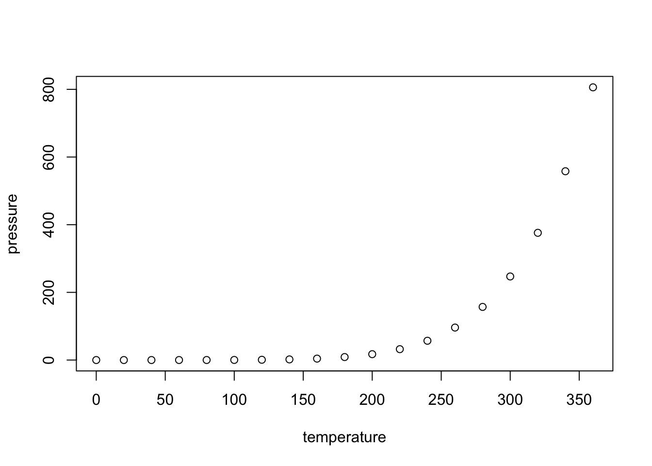
Note that the echo = FALSE parameter was added to the code chunk to prevent printing of the R code that generated the plot.
Demonstration: Pushing to Site
Participants curious about this website setup are encouraged to visit Like this setup? for notes on the resources I used.
Pushing new content to the live site consists of three steps: Knit, Commit, and Push.
Selecting Knit HTML  in the console opens a live preview window. If I had an RPub account synced to this console, I could select Publish
  and automatically send the generated HTML document to an RPub website. My configuration, however, requires two quick additional steps.
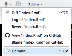
We commit changes in the Version Control dropdown menu:
The left pane displays files that have been changed. Now we select Staged for all of them and add a useful commit message. We select Commit, close the confirmation window, and finally push the content to the site with Push.
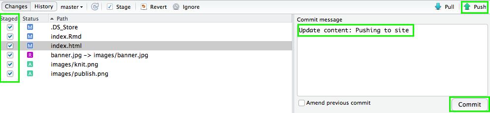
Interesting to note: Occasionally, the commit will fail the first time, but succeed on a second attempt. Cursory reserach reveals that this is not an uncommon issue, but I have not yet uncovered the reason. As it does not occur in my home, it may possibly have to do with FSU’s campus firewalls.
We can quickly browse the available references (see Reference Links in the Initial Setup section) to get an idea of what RMarkdown can do. A significant note here is that, while this is an HTML website, RMarkdown has several other output formats available including presentations, word processing and PDF documents, notebooks, and interactive content. This last output is what I want to explore in today’s Percolator session.
Shiny Web Apps
Adding runtime: shiny to the YAML head (which is actually not the same Pandoc markdown language we are using in the rest of the document) allows us to call Shiny code right in the document. Once we do so, we can see that the Knit HTML option has changed to Run Document  .
.
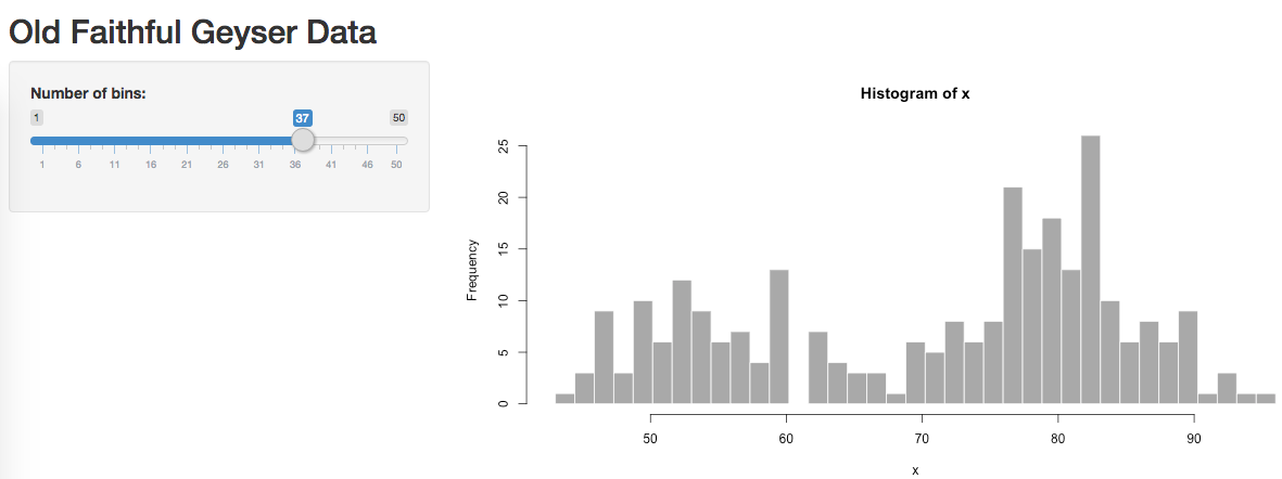
We first open a standalone Shiny app in RStudio to get an idea of how it behaves: File -> New File -> Shiny Web App… We select Run App  to run the auto-generated web application the sample text provides, which opens in an interactive preview window:
Now we’re playing! It’s time to call some Shiny code into RMarkdown. I take the sample code from the RMarkdown Cheatsheet and pop it into our newly-minted Shiny Web Apps section.
{r, echo = FALSE}
numericInput("n",
"How many cars?", 5)
renderTable({
head(cars, input$n)
})
We can play around with the cars app in the preview window, but here we run into publishing issues. Because Run Document has completely replaced the option to knit an HTML document, we cannot publish this to the site. Returning to our reference documents, we see that Shiny apps are server-side and, as browsers do not read R code, only run in an active R session. I take runtime: shiny out of the head so that I can knit the final results, supposing that the browser version will display a static screenshot. Instead RStudio calls an error: without runtime: shiny, it cannot call the code at all:
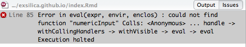
I’ve instead changed the app markup to unexcuted code (what you see above) to display what we tried to run. It appears the best solution is to create a shinyapps.io account to publish my web apps, and link to them from there. I’ll set that up in the following week, and in next week’s session we can focus on navigating shinyapps.io as well as client-side htmlwidgets.
Thank you Sarah, Nicole, and Bryan for a fun and informative exploratory session!
R & RStudio Setup
I made a Research Guide covering installation, setup, the RStudio environment, and some quick tips. I will continue to update it based on the type of questions we get.
Powered by RMarkdown and GitHub Pages.
